Real-Time Leaf Detection Using Stereo Camera
Overview:
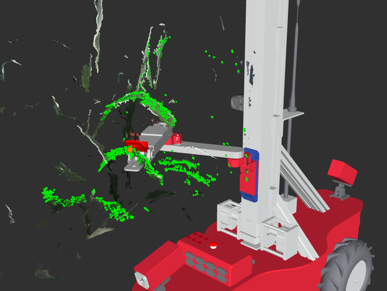
As part of my robotics research at Carnegie Mellon, I developed a computer vision pipeline to quickly and reliably detect crop leaves in real-time from images taken by our group's mobile agricultural robot. These computer vision algorithms take in stereo images of sorghum (or corn) and outputs a simplified, three dimensional model of the stalks and leaves within the scene. A Multisense S7 stereo camera by Carnegie Robotics is rigidly mounted to the side of the vertical mast of the mobile robot base and provides dense 3D range data of the environment. The Multisense S7 begins by capturing simultaneous images from right and left cameras and uses an onboard FPGA to perform rapid correspondence matching between images to calculate distance values for points in the scene. Through this process, the Multisense can output depth maps and colored point clouds at up to 15 fps. An example of a set of stereo images from the Multisense as well as the resulting point cloud can be seen below.

Leaf Detection Pipeline:
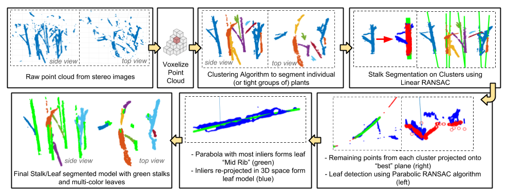
The leaf detection pipeline begins by creating a voxelized representation of the raw point cloud. This method significantly reduces the number of points in the cloud by instead storing only the centroids of points within small discretized 3D volume elements. This voxel grid is then converted into a k-d tree using the Point Cloud Library (PCL), a form of binary search tree that dramatically speeds up searching for points throughout space. A clustering algorithm is then employed, using the k-d tree for added efficiency, to detect and store large groups of points using a 2 cm distance threshold. Only clusters consisting of a certain number of points, in this case 100 points, are saved for later processing.
The next stage of the pipeline works to identify stalks within these large clusters through the use of an iterative linear random sample consensus (RANSAC) algorithm. Ultimately, all points belonging to stalks will be segmented out of the cloud in order to simplify the search for leaves. The linear ransac algorithm attempts to find one or more 3D line(s) that best fit the data within each cluster while ignoring potential outliers. This linear RANSAC algorithm for stalk segmentation is discussed in much more detail in the section below. For each cluster, all of the points that are not determined as inliers to a detected stalk are retained while the stalk inlier points are segmented out.
At this point in the pipeline, the clusters now represent a significantly downsampled version of the original point cloud where all stalk points as well as noisey outlier points have been removed. Thus, the existence of leaves should now be much easier to detect. Next, another RANSAC style algorithm is used that attempts to fit parabolic leaf models to the remaining points. A second order polynomial functions as an accurate model for sorghum leaves given the natural curvature. The details of this parabolic RANSAC leaf detection algorithm are discussed in much more detail in the section below. The inliers of a successful parabolic leaf model are considered to be points that belong to a leaf in the scene. Furthermore, the inliers projected onto the parabolic model form a clean parabola in 3D space that cuts through the middle of each leaf to form a sort of virtual leaf midrib. The inliers from both the linear stalk detection and parabolic leaf detection algorithms can be plotted together to form a clean 3D model of all the sorghum stalks and leaves from the original scene, as shown in the pipeline figure above.
Basic Stalk Segmentation Using Linear RANSAC:

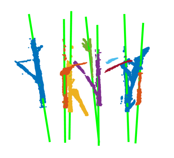
Example of Detected Stalks Using Linear RANSAC
As stated in the previous section, stalk segmentation is performed using a RANSAC algorithm that attempts to fit a line to each cluster by maximizing the number of points within a certain threshold distance while ignoring outliers in the data. The random nature of a RANSAC algorithm makes it non-deterministic, however, it is often run many thousands of times to ensure an accurate model is found. The steps of the linear RANSAC stalk detection algorithm are detailed below.
- Linear RANSAC Stalk Detection Algorithm
- Two points within the cluster are randomly selected to uniquely define a line in 3D space and
the
model parameters
(ax + by + c = 0)are derived and stored. - The angle between the the normal vector of the ground plane and the line is found. If the angle is greater than the vertical angle threshold then the current iteration is over and step 1 is repeated.
- For all other points in the cluster, find the Euclidean distance to the line. If the distance is less than the distance threshold, then the point is stored in a current list of inliers.
- If the number of inliers is greater than the number of inliers from the previous best model as well as the specified minimum model size, then the current model is stored as the best model.
- Repeat steps 1-4 until the total number of iterations has been reached.
- The model parameters of the line with the most inliers are used to represent a stalk. The algorithm is repeatingly run on the set of outliers from the previous result until there are no more stalks found in the cluster that meet the minimum model size constraint.
The value of key parameters used throughout the algorithm can be seen below:
- Key Parameters in the Stalk Detection Algorithm
- Number of Iterations: 10,000
- Vertical Angle Threshold: 10 degrees
- Distance Threshold: 1 cm
- Minimum Model Size: 75 points
Detecting Leaves Using Parabolic RANSAC:

Example of Detected Leaves Points (light green) Overlaid on Raw Point Cloud
The Parabolic RANSAC leaf detection algorithm is similar in principle to the linear RANSAC method described above. In essence, the algorithm attempts to find the set of model parameters, in this case for a parabola, that maximize the number of inliers in a cluster of points. However, the key difference with this algorithm is in the complexity of solving for the model parameters given a random set of points. Intuitively, it may seem as though three randomly selected points would define a unique parabola in three dimensional space much like three points can define a parabola in two dimensional space, however, this is far from the case. In two dimensions, three points of the form (x,y) only uniquely define a parabola given the constraint that the parabola is a function of y in terms of x, and thus has an axis of symmetry parallel with the y-axis. Without this constraint, a set of three points can be fit by an infinite number of parabolas in most cases. Therefore, in order for a set of three points to uniquely represent a single parabola, the plane on which the parabola will lie as well as a vector specifying the direction of the axis of symmetry must be given.
The general shape and orientation of sorghum leaves can be used to help form these constraints. Primarily, it can be noted that the midrib of almost all sorghum leaves lies on a plane that is perpendicular to the ground plane. In other words, from a top down view of the leaf, the midrib does not appear to curve at all. Furthermore, it is almost always the case that the point of inflection along a leaf’s midrib is also the highest point on the leaf (or the point furthest from the ground plane). This would mean that a parabolic representation of a leaf would have an axis of symmetry very close to the vertical vector. For these two reasons, all parabolic leaf models are constrained to planes that are perpendicular to the ground plane while also having axes of symmetry equal to the vertical vector.
- Parabolic RANSAC Leaf Detection Algorithm
- The constrained plane in which all points within the cluster will be projected is found.
- A basic linear RANSAC algorithm is run on the cluster with no angle constraint, a distance threshold of 1 cm, and a minimum model size of 20 points for a total of 10,000 iterations. This line is used to find a directional unit vector that roughly points along the length of the leaf.
- The normal vector of the constrained plane is found using the cross product of the directional unit vector of the leaf and the vertical vector.
- A point on the plane is found using the centroid of the inliers from the linear RANSAC in part 1a. Together, the point and normal vector fully define the constrained plane.
- All of the points in the cluster are projected onto the surface of the constrained plane, and the associated Euclidean distances from each point to the plane are also stored.
- A rotation matrix that rotates the constrained plane to be parallel with the XZ plane is found and the set of projected points are rotated to zero out the y-components for ease of future calculations.
- Three points on the plane are randomly selected and the model parameters for a unique parabola are found given the vertical axis of symmetry constraint. The parabola must be concave down (to represent a physically accurate leaf) or else step 4 is repeated.
- For all points on the plane, the Euclidean distance to the parabola is found. The total distance value for each point is equal to the projected distance from the original point to the plane plus the distance from the projected point to the parabola. If the total distance is less than the distance threshold, then the point is stored in a current list of inliers.
- If the number of inliers is greater than the number of inliers from the previous best model as well as the specified minimum model size, then the current model is stored as the best model.
- Repeat steps 4-6 until the total number of iterations has been reached.
- The inliers from the best model are rotated back using the inverse rotation matrix found in step 3. The projected inliers form a clean parabola that resembles the leaf midrib while the reprojected inliers form all points along the detected leaf surface.
- The algorithm is repeatingly run on the set of outliers from the previous result until there are no more leaves found in the cluster that meet the minimum model size constraint.
The value of key parameters used throughout the algorithm can be seen below:
- Key Parameters in the Leaf Detection Algorithm
- Number of Iterations: 2,000
- Distance Threshold: 8 cm
- Minimum Model Size: 60 points
After running this parabolic RANSAC algorithm to completion on all of the clusters, a full model of all stalks and leaves in the original scene should now be extracted. This is the last stage of the leaf detection pipeline, however, the parabolic leaf models will now be used to detect optimal grasp points for the robotic manipulator.