Extended Kalman Filtering for State Estimation with Noise
Overview: This project is an extension of 3D State Estimation and Control as it deals with estimating the state of an “alien artifact” tumbling through space. However, here we focus on state estimation in the presence of sensor noise and occlusion. The goal is to use an Extended Kalman filter to produce optimal estimates of the position, orientation, and velocity of the artifact using noisy data of the markers on the corners of the artifact.
Source Code: https://drive.google.com/open?id=0B81gni53B9VOOENQWGgzanR4ak0
Setup:
As described above, the goal of this project is to estimate the state and future trajectory of a rectangular object as it tumbles through space. In order to do so, all we are given a text file containing 10 seconds of position data of markers on all corners of the object. However, this data is rather noisy making traditional state estimation techniques useless. Instead, we will employ an Extended Kalman Filter to estimate the true state of the artifact as it tumbles through space.
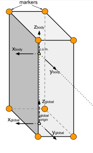
A diagram of the alien artifact (with markers on its corners) as well as our lander spacecraft is shown below.
Modeling the State Space:
As estimating the state involves estimating angular velocities (and orientation representation in quaternions), we are going to be dealing with non-linear dynamics. However, a Kalman filter is based on linear dynamic systems, so we can begin by creating our state estimate vector that we will use to eventually create a linearized representation of our dynamic system (the tumbling artifact that is). Because we need to track the COM position and velocity as well as the artifact orientation and angular velocity, my state estimate vector includes all of these terms. However, I initially represent the artifact orientation in terms of Euler angles as they correlate much nicer to the angular velocity terms than quaternions, but I convert these angles into quaternions at a later point. Here is my state estimate vector (where ax, ay, az are Euler angles):

Creating the State Space System: Because a Kalman filter is based on linear system dynamics, we ideally need the dynamics of the artifact to be represented by a linear system of the following form:
x(k+1) = A*x(k) + B*u(k)
Where A represents the state matrix (from the system dynamics), x represents the state vector, B represents the input/control matrix, and u represents the input/control vector. We begin by solving for the next state in time, x(k+1), given our current state, x(k), and a time step, T:
x(k+1)  = x(k) + T * dx(k);
y(k+1)  = y(k) + T * dy(k);
z(k+1)  = z(k) + T * dz(k);
dx(k+1) = dx(k);
dy(k+1) = dy(k);
dz(k+1) = dz(k);
ax(k+1) = ax(k) + T * ωx(k);
ay(k+1) = ay(k) + T * ωy(k);
az(k+1) = az(k) + T * ωz(k);
The above equation take care of the first 9 states in the state vector, and the best part is that they are all linear equations. We run into a problem when we try to solve for the future state of the last three variables (ωx, ωy, ωz). Like above, we need information about a state variables derivative to step forward in time and estimate the state at k+1. From rigid body dynamics, we can solve for the artifact’s angular acceleration using the following equation of motion:
T = I * α + (ω x I * ω)
where:
T = applied torque
I = moment of inertia matrix
α = angular acceleration
ω = angular velocity
Given that the artifact has no external applied torques, we can set the above equation equal to zero and solve for α (the derivative of angular velocity):
α = -inv(I) * (ω x I * ω)
Note: All of the above variables should be represented in the global frame. As I describe below, I track α and ω in the global frame, however, we are only given I (the moment of inertia matrix) in body coordinates along its principal axes. In order to orient the body fixed moment of inertia matrix in the global frame, we can convert our current orientation (in quaternions) into a rotation matrix, Rq, using quat2rotm() in MATLAB. Next, we can simply rotate the I_body matrix into the global frame by the following:
I_global = Rq * I_body * Rq'
This output, angular acceleration, is exactly what we are looking for as it represents the derivatives of the angular velocity components (ωx, ωy, ωz). However, there is a significant problem here, and it is that the above equation for α is non-linear with respect to our state variables. Because of this fact, we cannot easily lump our equations for the future state of the system into the convenient form x(k+1) = A*x(k) + B*u(k) and use the typical Kalman filter design. In order to solve this problem, we must create a non-linear version of the Kalman filter known as the Extended Kalman Filter. To do this, we essentially linearize our model about our current state estimate and covariance. Instead of the linear form x(k+1) = A*x(k), we have a state space model of the form:
x(k+1) = f(x(k))
where f() is a non-linear function that maps the current state estimate, x(k), to the next state, x(k+1). We can approximate this function by calculating the functions Jacobian matrix, F, which is a matrix that contains all first order partial derivatives of the function, f(). The partial derivatives are evaluated with the current state information to obtain a linear first order approximation of the system of the form:
x(k+1) = F * x(k)
Creating the Extended Kalman Filter:
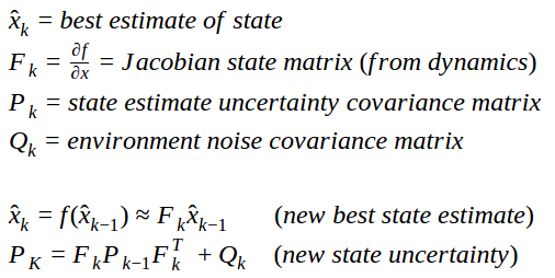
Now that we have a model for ‘linear’ dynamics around our current state estimate vector, we can begin forming the structure of the Extended Kalman filter. Similar to any linear state space model, we can predict the state at some time step k given the previous state at time k-1 and our Jacobian state matrix, F, that represents the dynamics of our system. This relation can be seen in the first equation shown below (new best state estimate). However, there is always some uncertainty that goes along with any state estimate, and we can represent this with a state uncertainty covariance matrix, P. Furthermore, there is added noise from the environment which can be represented by an environmental noise covariance matrix, Q. Thus the new state uncertainty, P(k), can be solved for with the second equation below:
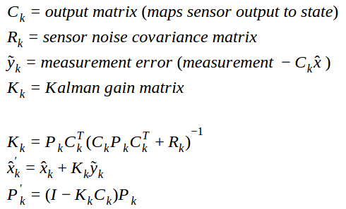
The above equations represent the prediction step. With those equations and knowledge of the previous state, x(k-1) and P(k-1), we can obtain our best estimate of the new state as well as the uncertainty of said state. Next, we can refine or update our state estimate using the marker data. In order to get our state into the form of our measurement output, we need what’s called an output matrix, C. This maps variables in our state to an output vector that is in a similar form as the measurement data (marker data) we have. Just like in the prediction step, we must represent the uncertainty due to sensor noise with a covariance matrix, R. With all of this information, we can now solve for our Kalman gain matrix, K, which helps us solve for a final and optimal state estimate, x’. Using the Kalman gain matrix, we can pre-multiply it by our measurement error to then add to our current best state estimate from the prediction step. This yields our final best state estimate at time k. We must also update our state uncertainty matrix, P, using the Kalman gain. The equation to do so is also shown below:
With an initial state as the input to the Extended Kalman filter, we can then repeat the process above for all steps in time until we reach some desired final state.
Below is the output from my Extended Kalman Filter for the first set of noisy marker data provided.

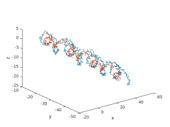
Noisy Position of Top 2 Markers

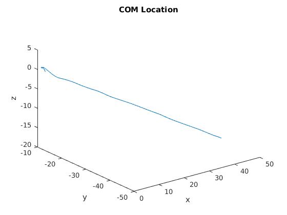
Estimated COM Trajectory
In the left image, only the noisy Marker 0 and Marker 1 (along the back right vertical edge, body z-axis) data is plotted so we can see the rough tumbling shape of the artifact. In the right image, the COM position output from the EKF is plotted. We can see that the estimated COM position lies nicely through the noisy marker data trajectory and does not deviate from a straight line as there are no external forces acting on the artifact.
The estimated center of mass velocity as well as the estimated angular velocity (in all three components) is also plotted below:
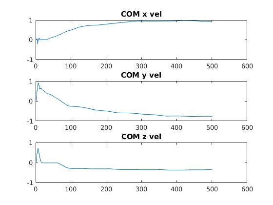
Estimated COM Velocity
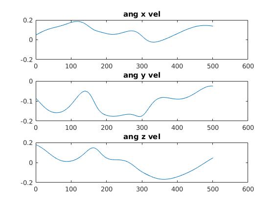
Estimated Angular Velocity
Lastly, the estimated quaternion orientation is plotted below (broken down to the 4 components):
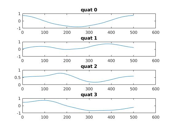
Estimated Quaternion Orientation