Inverse Kinematics Using Optimization

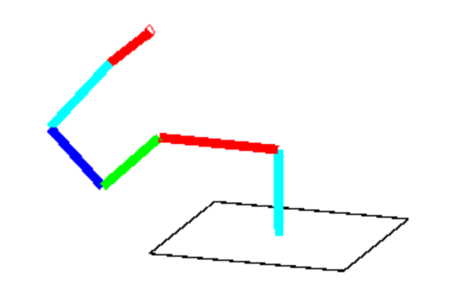
Overview: Through the use of function optimization in MATLAB, the position and orientation of a 3-dimensional snake robot is controlled in order to reach into an environment and grasp an object. The snake robot consists of a serial chain of kinematic links, of arbitrary number and length, where each joint is controlled with a set of Euler angles (roll, pitch, yaw). The environment is filled with spherical obstacles that the robot must avoid in reaching the obstacle.

Source Code: https://drive.google.com/open?id=0B81gni53B9VORVJNUGxWQ0F1cFk

Setup:

Objective: Write a MATLAB program (part1.m) to position control the tip of the robot (end of the last link) to a specified location and orientation. The position is given as a set of Cartesian coordinates [x, y, z] while the orientation of the last link is given as a quaternion [q0, q1, q2, q3].

Function Inputs:

The target, given as (x, y, z, q0, q1, q2, q3)
A vector of link lengths (of size Nx1 for a total of N links)
Limits on the roll, pitch, and yaw angles of each link
A series of spherical obstacles given as (x, y, z, radius)

Function Outputs:

Roll, Pitch, and Yaw vectors for all N links to position the tip at the given target
A graphical animation of the robot as it searches for the target

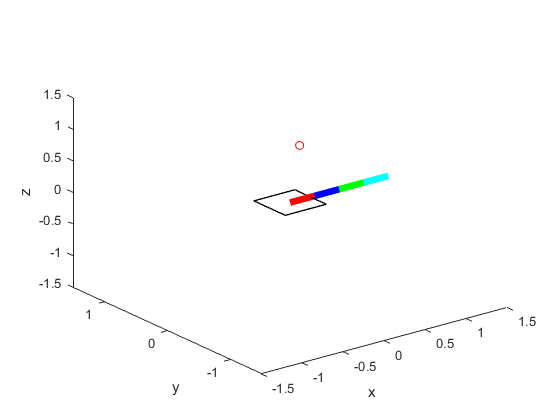
Home Position

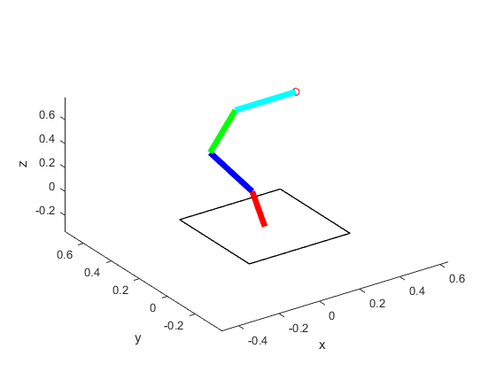
Example Configuration That Reaches Target

Solving Inverse Kinematics:

The actual optimization process was done using the function fmincon in MATLAB. Essentially, fmincon takes some initial set of joint angles for each link and continuously attempts to find a new set of angles that minimizes a cost function until a set of constraints (desired tip location and orientation) is achieved within a certain accuracy. Therefore, we must develop a cost function (criterion.m) that the program will attempt to minimize as well as a series of constraints (constraints.m) that must be obeyed in the optimization.

part1.m acts as the main function that initializes global variables for the desired target, link lengths, and the home position of the robot (to be used in the cost function). First, a variable p0 is initialized with all zero Euler angles for all links to represent the home position which will be used as the initial set of angles for the optimization function. Next, the angle limit constraints are organized into lower and upper bounds (lb and ub respectively) for the matrix of joint angles to be passed into fmincon. Finally, the optimization function, fmincon, is called using the local function criterion.m as the objective cost function and the function constraints.m to specify the desired location and orientation constraints. The ‘interior-point’ algorithm is used as default with a maximum of 1000 function evaluations as shown below:

options = optimset('Display','iter','MaxFunEvals',10000,'Algorithm','interior-point');

[answer,fval,exitflag] = fmincon(@criterion,p0,[],[],[],[],lb,ub,@constraints,options);

criterion.m is the next function that is called by fmincon. This function takes in a matrix of Euler joint angles for each link and then performs Forward Kinematic calculations to derive the location and orientation of the last link using a function I wrote called fk.m (see description of fk.m below for more details). Now with the position of the last link, a cost function is created that calculates the square of the Euclidean distance between the tip and the desired location as well as the deviation of each joint angle from its home position (to encourage a solution that requires the least amount of link rotation/movement). A gain is multiplied by each of these two quantities before summing them as a way to tune the performance. I ended up applying a much larger gain to the squared Euclidean distance as it is more crucial and I found it decreased run time.

constraints.m is the second function that controls the optimization process of fmincon. Here, a series of nonlinear equality and inequality constraints are formulated that must be achieved within a given accuracy range before fmincon returns a minimum solution. The equality constraints specify that the location and orientation of the tip must equal the desired location and orientation. The current orientation of the last link is calculated from the vector along the previous link's x-axis. The orientation is compared to the given quaternion in the constraint equation by first converting the quaternion to a rotation matrix (using MATLAB’s quat2rotm function) and then constraining the unit projection of the last link vector on the first column of the rotation matrix to be 1.

Equality Constraints:

eq_violations(1) = pos(end, 1) - x_d(1);
eq_violations(2) = pos(end, 2) - x_d(2);
eq_violations(3) = pos(end, 3) - x_d(3);
rotm = quat2rotm(desired_quaternion_orientation');
eq_violations(4) = sum((link_vec' - rotm(:,1)).^2);

Avoiding Obstacles:

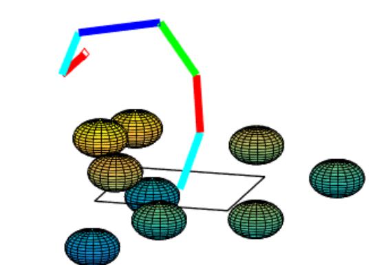
A random set of spherical obstacles is now placed in the environment, and the robot must now reach its goal pose while avoiding these obstacles. In order to do so, inequality constraints are used to ensure that the links do not intersect or collide with the spherical obstacles. Here, the link end points are constrained so that they do not fall within the bounds of each sphere. These inequality constraints are placed within the constraints.m function.

Inequality Constraints:

%Note: r= sphere radius, (x,y,z) = sphere center
%Note: j = sphere number, k = link number
ineq_violations((j-1)*length(l)+k) = r^2 - (pos(k,1)-x)^2 - (pos(k,2)-y)^2 - (pos(k,3)-z)^2;

Demonstration:

In order to demonstrate the robot's ability to avoid obstacles, we can first construct an environment with no obstacles and the following goal state: [x,y,z,q0,q1,q2,q3] = [0.5,0.5,0.5,1,0,0,0]

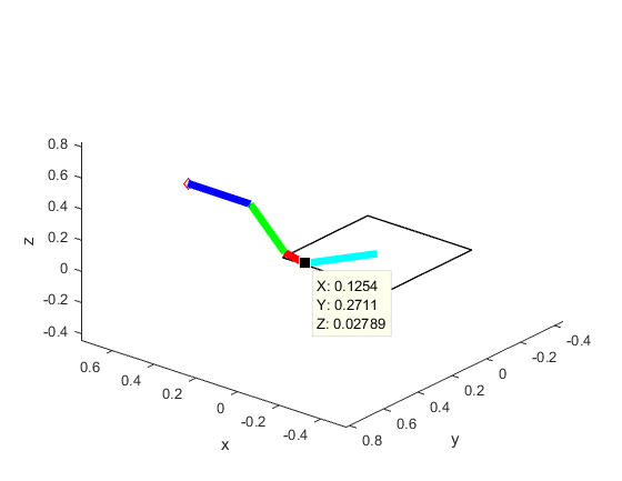
Successful pose before adding interfering sphere

Now we add a spherical obstacle at [0.125, 0.271, 0.028] with radius 0.2 to see if the robot avoids the obstacle.

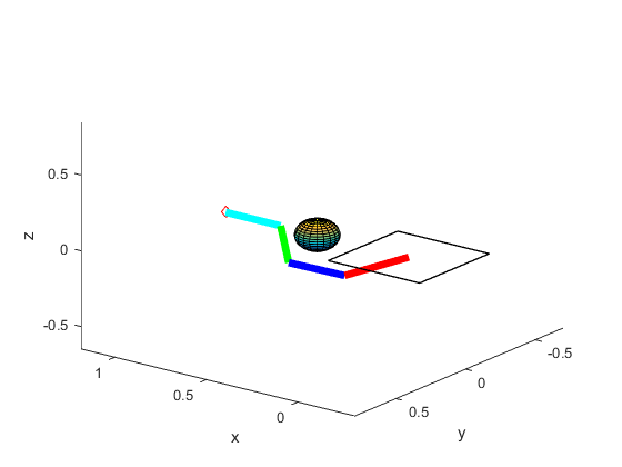
Robot reaches goal with new orientation to avoid sphere

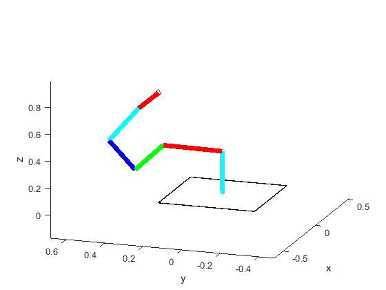
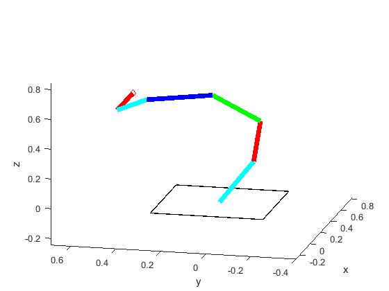
Gallery:

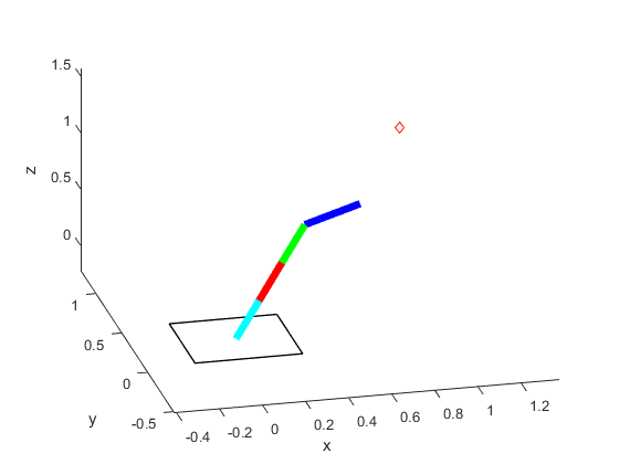
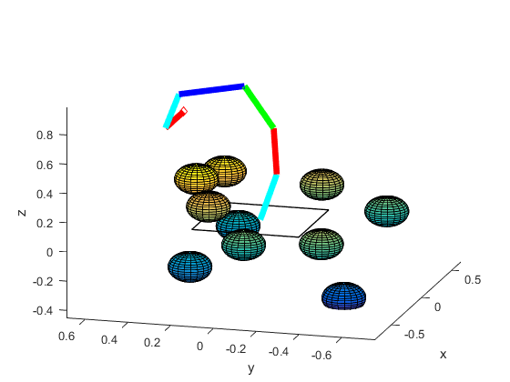
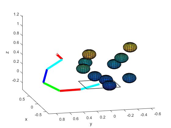
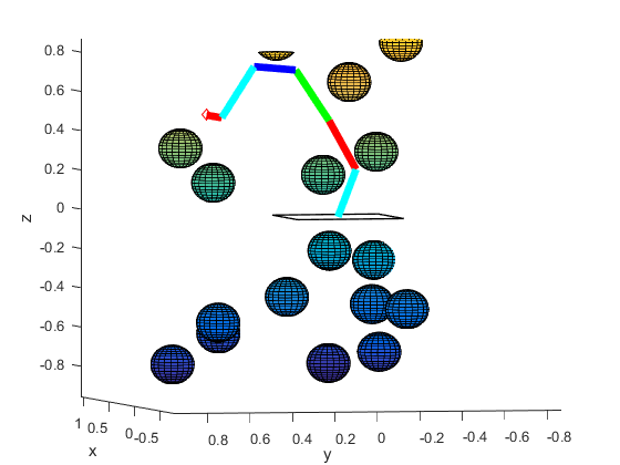
Appendix: Forward Kinematics

fk.m takes the matrix of joint angles for each link and returns the position of each link using forward kinematics. The function loops through each link and calculates the relative rotation matrix, compared to the previous link. This rotation matrix is formed by multiplying the Rx (roll), Ry (pitch), and Rz (yaw) rotations together as shown below. Then the total rotation matrix is multiplied by the relative coordinates of the end of the current link [link_len 0 0]’ and added to the coordinates of the previous link.


% r(i) = roll, p(i) = pitch, y(i) = yaw;
Rx = [[1          0          0         ];
      [0          cos(r(i))  -sin(r(i))]
      [0          sin(r(i))  cos(r(i)) ]];
Ry = [[cos(p(i))  0          sin(p(i)) ];
      [0          1          0         ];
      [-sin(p(i)) 0          cos(p(i)) ]];
Rz = [[cos(y(i))  -sin(y(i)) 0         ];
      [sin(y(i))  cos(y(i))  0         ];
      [0          0          1         ]];
Rtot = Rx*Ry*Rz;
Rtot = Rprev*Rtot;
[cur_x cur_y cur_z]' = Rtot*[link_len 0 0]' + [prev_x prev_y prev_z]'

Appendix: Drawing the Robot

draw.m is called within the criterion.m function in order to show a graphical representation of the current orientation of the robot as fmincon attempts to find a set of joint angles that minimizes the cost function while achieving the constraints. draw.m calls fk.m to retrieve the current position of each link and then uses the MATLAB function plot3 to plot lines in 3D space that represents each link. This function also uses the target location (saved as a global variable) to plot a small red circle to represent the desired location of the tip of the last link.